#imports
import os
import tensorflow as tf
from tensorflow import keras,strings
from tensorflow.keras import utils
from tensorflow.keras import layers,losses
import pandas as pd
import re
import string
from sklearn.decomposition import PCA
from matplotlib import pyplot as plt
from plotly import express as px
import plotly.io as pio

pio.renderers.default= 'colab'

tf.config.run_functions_eagerly(True)For this assignment we’re using Tensorflow (again!) to make a fake news classifier. Like always, we start with all the imports we’ll be using throughout the project.
Data Preparation
We’ll be using a dataset of news articles that includes their title, text content, and whether or not they contain fake news. The data from the below URL is training data only; we’ll be importing the testing data once we have a decent running model.
#import training data
train_url = "https://github.com/PhilChodrow/PIC16b/blob/master/datasets/fake_news_train.csv?raw=true"
df = pd.read_csv(train_url)df.head()| Unnamed: 0 | title | text | fake | |
|---|---|---|---|---|
| 0 | 17366 | Merkel: Strong result for Austria's FPO 'big c... | German Chancellor Angela Merkel said on Monday... | 0 |
| 1 | 5634 | Trump says Pence will lead voter fraud panel | WEST PALM BEACH, Fla.President Donald Trump sa... | 0 |
| 2 | 17487 | JUST IN: SUSPECTED LEAKER and “Close Confidant... | On December 5, 2017, Circa s Sara Carter warne... | 1 |
| 3 | 12217 | Thyssenkrupp has offered help to Argentina ove... | Germany s Thyssenkrupp, has offered assistance... | 0 |
| 4 | 5535 | Trump say appeals court decision on travel ban... | President Donald Trump on Thursday called the ... | 0 |
In natural language processing it’s common to remove stopwords, a set of commonly used neutral words in the language, from input data. This allows our models to spend more energy analyzing meaningful words. We can download a set of English stopwords from the nltk package.
Here, we implement this preprocessing as part of make_dataset(), which deletes stopwords from a given dataframe and turns it into a Tensorflow Dataset object. This is achieved using the from_tensor_slices() function. To allow for multiple inputs to be processed later, we pass a tuple of dictionaries, where the first dictionary corresponds to text and title inputs and the second dictionary correspond to the label, or the output of whether or not the corresponding article contains fake news.
Finally, we batch the function for increased training speed before returning it.
import nltk
nltk.download('stopwords')

from nltk.corpus import stopwords
stop = stopwords.words('english')

def make_dataset(df):
    df = df.copy()

    drop_stopwords = lambda words: ' '.join(word.lower() for word in words.split() if word not in stop)

    #drop stopwords from title and text columns
    df["title"] = df["title"].apply(drop_stopwords)
    df["text"] = df["text"].apply(drop_stopwords)

    #create and batch dataset from dataframe
    data_set = tf.data.Dataset.from_tensor_slices(({"title":df[["title"]],"text":df[["text"]]}, {"fake":df[["fake"]]}))
    data_set = data_set.batch(100)
    return data_set
[nltk_data] Downloading package stopwords to /root/nltk_data...
[nltk_data] Unzipping corpora/stopwords.zip.data = make_dataset(df)Next, we split 20% of our data to be used as validation data, and use the remainder to train our model.
#separate 20% of data as validation data

val_size = int(0.2*len(data))

val = data.take(val_size)
train = data.skip(val_size)
Let’s take a look at the distribution of fake news in our dataset to determine the base rate. Like with Homework 4, we construct an iterator that allows us to extract the “fake” column of our dataset and use some list functions to determine the number of fake and true articles.
labels_iterator = train.unbatch().map(lambda data_dict,fake: fake["fake"]).as_numpy_iterator()/usr/local/lib/python3.9/dist-packages/tensorflow/python/data/ops/structured_function.py:256: UserWarning:
Even though the `tf.config.experimental_run_functions_eagerly` option is set, this option does not apply to tf.data functions. To force eager execution of tf.data functions, please use `tf.data.experimental.enable_debug_mode()`.
WARNING:tensorflow:From /usr/local/lib/python3.9/dist-packages/tensorflow/python/autograph/pyct/static_analysis/liveness.py:83: Analyzer.lamba_check (from tensorflow.python.autograph.pyct.static_analysis.liveness) is deprecated and will be removed after 2023-09-23.
Instructions for updating:
Lambda fuctions will be no more assumed to be used in the statement where they are used, or at least in the same block. https://github.com/tensorflow/tensorflow/issues/56089#count fake and true news articles in dataset
labels = [i for i in labels_iterator]
num_fake = sum(labels)
num_true = len(labels) - num_fake
print(num_fake,num_true)[9412] [8537]There are 9412 articles containing fake news and 8537 without, so the base model will guess that a given news article is fake with probability \(\frac{9412}{9412+8537} \approx 52.4\%\), which is the base rate.
Creating Models
Before we assemble models using the Tensorflow Functional API, we need to prepare some layers. Most neural network layers can’t immediately process text, so we need to convert text to integer sequences before they can be interpreted and analyzed. The TextVectorization layer object does this for us. For the purposes of this model we use a size_vocabulary of 2000 (this tells the layer to focus on the 2000 most meaningful distinct words) and output_sequence_length of 500. Furthermore, we can add a standardization parameter that in our case lowercases and removes punctuation from all text through the standardization() function.
We make two layers; one for interpreting article titles and one for interpreting article contents. Once created, each layer can be adapted to their respective data inputs.
#prepare TextVectorization layers for both title and text inputs
size_vocabulary = 2000

#more preprocessing
def standardization(input_data):
    lowercase = tf.strings.lower(input_data)
    no_punctuation = tf.strings.regex_replace(lowercase,
                                  '[%s]' % re.escape(string.punctuation),'')
    return no_punctuation

title_vectorize_layer = layers.TextVectorization(
    standardize=standardization,
    max_tokens=size_vocabulary, # only consider this many words
    output_mode='int',
    output_sequence_length=500)

#adapt layer to title vocabulary
title_vectorize_layer.adapt(train.map(lambda x, y: x["title"]))

text_vectorize_layer = layers.TextVectorization(
    standardize=standardization,
    max_tokens=size_vocabulary, # only consider this many words
    output_mode='int',
    output_sequence_length=500)

#adapt layer to text vocabulary
text_vectorize_layer.adapt(train.map(lambda x, y: x["text"]))
In Homework 4, we used Tensorflow’s Sequential API to construct neural networks. The limitation there is that the sequence of layers is strictly linear. In reality, however, neural networks are often closer to a directed graph, where layers can branch off, be reused, and accept multiple inputs. The Functional API better implements this.
To create a model using the Functional API, we start by defining Input objects. In particular these take in a name parameter that corresponds to keys in the dictionaries in our dataset.
#create inputs
title_inputs = keras.Input(shape=(1,),name="title",dtype="string")
text_inputs = keras.Input(shape=(1,),name="text",dtype="string")
Our first model will only consider article titles. Along with Dropout(), which we used in Homework 4, and the title_vectorize_layer that we defined early, we introduce an Embedding() layer, which turns the integer sequences outputted by the vectorization layer and turns them into dense vectors, as well as a GlobalAveragePooling1D() layer, which averages data across one dimension. We complete the model by assigning a Dense() layer taking in previous layers to title_outputs, and then constructing title_model, a keras.Model object.
#model that takes in title only
x = title_vectorize_layer(title_inputs)
x = layers.Embedding(size_vocabulary,output_dim=3,name="embedding")(x)
x = layers.Dropout(0.1)(x)
x = layers.GlobalAveragePooling1D()(x)
title_outputs = layers.Dense(2,activation='softmax',name="fake")(x)
title_model = keras.Model(inputs=title_inputs,outputs=title_outputs)Here’s what our model looks like:
title_model.summary()Model: "model"
_________________________________________________________________
Layer (type) Output Shape Param #
=================================================================
title (InputLayer) [(None, 1)] 0
text_vectorization (TextVec (None, 500) 0
torization)
embedding (Embedding) (None, 500, 3) 6000
dropout (Dropout) (None, 500, 3) 0
global_average_pooling1d (G (None, 3) 0
lobalAveragePooling1D)
fake (Dense) (None, 2) 8
=================================================================
Total params: 6,008
Trainable params: 6,008
Non-trainable params: 0
_________________________________________________________________In fact, we can visualize this in the form of a directed graph using utils.plot_model(). Right now our model is entirely linear, though, so it won’t look very interesting.
utils.plot_model(title_model)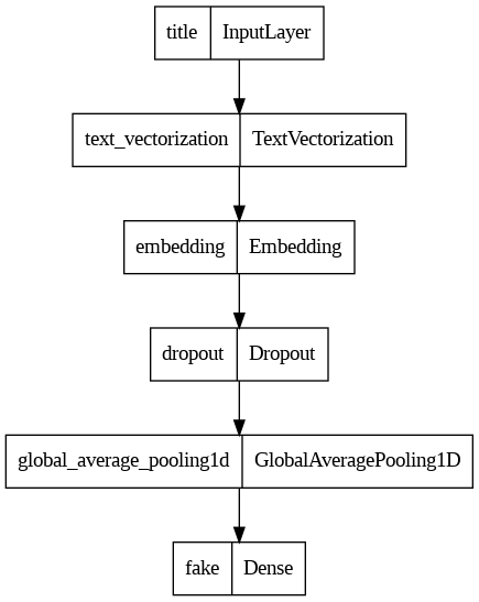
Now we can compile and train our model just like in the previous homework.
#compile model
sce = tf.keras.losses.SparseCategoricalCrossentropy(from_logits=False)

title_model.compile(optimizer='adam',
             loss = sce,
             metrics = ['accuracy'])
#train model on training data
title_history = title_model.fit(train,epochs=20,validation_data=val)Epoch 1/20/usr/local/lib/python3.9/dist-packages/keras/engine/functional.py:638: UserWarning:
Input dict contained keys ['text'] which did not match any model input. They will be ignored by the model.
180/180 [==============================] - 11s 40ms/step - loss: 0.6913 - accuracy: 0.5210 - val_loss: 0.6904 - val_accuracy: 0.5173
Epoch 2/20
180/180 [==============================] - 7s 38ms/step - loss: 0.6879 - accuracy: 0.5244 - val_loss: 0.6862 - val_accuracy: 0.5173
Epoch 3/20
180/180 [==============================] - 7s 40ms/step - loss: 0.6821 - accuracy: 0.5253 - val_loss: 0.6790 - val_accuracy: 0.5173
Epoch 4/20
180/180 [==============================] - 7s 38ms/step - loss: 0.6732 - accuracy: 0.5725 - val_loss: 0.6689 - val_accuracy: 0.5178
Epoch 5/20
180/180 [==============================] - 7s 41ms/step - loss: 0.6615 - accuracy: 0.6629 - val_loss: 0.6559 - val_accuracy: 0.5696
Epoch 6/20
180/180 [==============================] - 8s 44ms/step - loss: 0.6471 - accuracy: 0.7759 - val_loss: 0.6406 - val_accuracy: 0.6947
Epoch 7/20
180/180 [==============================] - 7s 40ms/step - loss: 0.6305 - accuracy: 0.8585 - val_loss: 0.6233 - val_accuracy: 0.8051
Epoch 8/20
180/180 [==============================] - 7s 38ms/step - loss: 0.6123 - accuracy: 0.9032 - val_loss: 0.6044 - val_accuracy: 0.8738
Epoch 9/20
180/180 [==============================] - 7s 41ms/step - loss: 0.5927 - accuracy: 0.9223 - val_loss: 0.5845 - val_accuracy: 0.9031
Epoch 10/20
180/180 [==============================] - 7s 40ms/step - loss: 0.5724 - accuracy: 0.9339 - val_loss: 0.5639 - val_accuracy: 0.9233
Epoch 11/20
180/180 [==============================] - 7s 38ms/step - loss: 0.5517 - accuracy: 0.9381 - val_loss: 0.5431 - val_accuracy: 0.9322
Epoch 12/20
180/180 [==============================] - 7s 41ms/step - loss: 0.5306 - accuracy: 0.9402 - val_loss: 0.5221 - val_accuracy: 0.9400
Epoch 13/20
180/180 [==============================] - 8s 42ms/step - loss: 0.5095 - accuracy: 0.9438 - val_loss: 0.5013 - val_accuracy: 0.9416
Epoch 14/20
180/180 [==============================] - 7s 37ms/step - loss: 0.4889 - accuracy: 0.9433 - val_loss: 0.4810 - val_accuracy: 0.9447
Epoch 15/20
180/180 [==============================] - 7s 40ms/step - loss: 0.4690 - accuracy: 0.9436 - val_loss: 0.4612 - val_accuracy: 0.9440
Epoch 16/20
180/180 [==============================] - 7s 41ms/step - loss: 0.4491 - accuracy: 0.9449 - val_loss: 0.4420 - val_accuracy: 0.9433
Epoch 17/20
180/180 [==============================] - 7s 37ms/step - loss: 0.4305 - accuracy: 0.9443 - val_loss: 0.4236 - val_accuracy: 0.9460
Epoch 18/20
180/180 [==============================] - 7s 40ms/step - loss: 0.4126 - accuracy: 0.9454 - val_loss: 0.4060 - val_accuracy: 0.9473
Epoch 19/20
180/180 [==============================] - 7s 41ms/step - loss: 0.3953 - accuracy: 0.9465 - val_loss: 0.3892 - val_accuracy: 0.9484
Epoch 20/20
180/180 [==============================] - 7s 38ms/step - loss: 0.3787 - accuracy: 0.9466 - val_loss: 0.3731 - val_accuracy: 0.9493
That’s a pretty impressive accuracy, and there doesn’t seem to be any overfitting! Let’s borrow our plot_accuracies() function from last time to visualize this.
def plot_accuracies(history,name):
    #plot validation accuracies of model with name
    accuracies = history.history["val_accuracy"]
    fig,ax = plt.subplots()
    ax.plot(range(1,len(accuracies)+1),accuracies)

    ax.set_title(name+" Fitting History")
    ax.set_xlabel("Epoch")
    ax.set_ylabel("Validation Accuracy")
    ax.set_xticks(range(1,len(accuracies)+1,2))

    return fig
title_plot = plot_accuracies(title_history,"Title Model")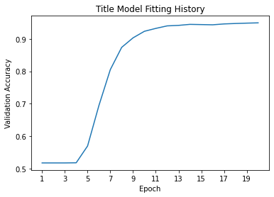
So it seems like just the title alone is a pretty good indicator of whether or not an article contains fake news, but can we do better? What if we considered the article’s contents instead? Our next model will be the same as the previous one, except it takes in text_inputs and uses the text_vectorize_layer instead.
#same process for text input only

#create model
x = text_vectorize_layer(text_inputs)
x = layers.Embedding(size_vocabulary,output_dim=3,name="embedding")(x)
x = layers.Dropout(0.1)(x)
x = layers.GlobalAveragePooling1D()(x)
text_outputs = layers.Dense(2,activation='softmax',name="fake")(x)

text_model = keras.Model(inputs=text_inputs,outputs=text_outputs)

#compile model
sce = tf.keras.losses.SparseCategoricalCrossentropy(from_logits=False)

text_model.compile(optimizer='adam',
             loss = sce,
             metrics = ['accuracy'])

#train model
text_history = text_model.fit(train,epochs=20,validation_data=val)
Epoch 1/20
3/180 [..............................] - ETA: 6s - loss: 0.6936 - accuracy: 0.4833 /usr/local/lib/python3.9/dist-packages/keras/engine/functional.py:638: UserWarning:
Input dict contained keys ['title'] which did not match any model input. They will be ignored by the model.
180/180 [==============================] - 8s 47ms/step - loss: 0.6820 - accuracy: 0.5343 - val_loss: 0.6686 - val_accuracy: 0.5596
Epoch 2/20
180/180 [==============================] - 8s 47ms/step - loss: 0.6467 - accuracy: 0.6862 - val_loss: 0.6231 - val_accuracy: 0.7462
Epoch 3/20
180/180 [==============================] - 8s 45ms/step - loss: 0.5938 - accuracy: 0.8483 - val_loss: 0.5651 - val_accuracy: 0.8567
Epoch 4/20
180/180 [==============================] - 8s 43ms/step - loss: 0.5339 - accuracy: 0.9059 - val_loss: 0.5058 - val_accuracy: 0.9027
Epoch 5/20
180/180 [==============================] - 8s 47ms/step - loss: 0.4765 - accuracy: 0.9232 - val_loss: 0.4524 - val_accuracy: 0.9184
Epoch 6/20
180/180 [==============================] - 9s 47ms/step - loss: 0.4265 - accuracy: 0.9292 - val_loss: 0.4074 - val_accuracy: 0.9251
Epoch 7/20
180/180 [==============================] - 8s 43ms/step - loss: 0.3849 - accuracy: 0.9339 - val_loss: 0.3703 - val_accuracy: 0.9331
Epoch 8/20
180/180 [==============================] - 8s 46ms/step - loss: 0.3505 - accuracy: 0.9372 - val_loss: 0.3399 - val_accuracy: 0.9389
Epoch 9/20
180/180 [==============================] - 9s 47ms/step - loss: 0.3221 - accuracy: 0.9412 - val_loss: 0.3148 - val_accuracy: 0.9409
Epoch 10/20
180/180 [==============================] - 8s 44ms/step - loss: 0.2981 - accuracy: 0.9435 - val_loss: 0.2937 - val_accuracy: 0.9438
Epoch 11/20
180/180 [==============================] - 8s 46ms/step - loss: 0.2778 - accuracy: 0.9475 - val_loss: 0.2758 - val_accuracy: 0.9460
Epoch 12/20
180/180 [==============================] - 8s 46ms/step - loss: 0.2602 - accuracy: 0.9506 - val_loss: 0.2602 - val_accuracy: 0.9476
Epoch 13/20
180/180 [==============================] - 8s 43ms/step - loss: 0.2453 - accuracy: 0.9535 - val_loss: 0.2468 - val_accuracy: 0.9493
Epoch 14/20
180/180 [==============================] - 8s 46ms/step - loss: 0.2318 - accuracy: 0.9553 - val_loss: 0.2349 - val_accuracy: 0.9507
Epoch 15/20
180/180 [==============================] - 8s 47ms/step - loss: 0.2197 - accuracy: 0.9570 - val_loss: 0.2244 - val_accuracy: 0.9522
Epoch 16/20
180/180 [==============================] - 8s 46ms/step - loss: 0.2094 - accuracy: 0.9584 - val_loss: 0.2150 - val_accuracy: 0.9524
Epoch 17/20
180/180 [==============================] - 8s 45ms/step - loss: 0.1993 - accuracy: 0.9611 - val_loss: 0.2065 - val_accuracy: 0.9547
Epoch 18/20
180/180 [==============================] - 8s 43ms/step - loss: 0.1903 - accuracy: 0.9623 - val_loss: 0.1988 - val_accuracy: 0.9564
Epoch 19/20
180/180 [==============================] - 8s 46ms/step - loss: 0.1820 - accuracy: 0.9641 - val_loss: 0.1918 - val_accuracy: 0.9571
Epoch 20/20
180/180 [==============================] - 8s 47ms/step - loss: 0.1748 - accuracy: 0.9650 - val_loss: 0.1854 - val_accuracy: 0.9589
text_plot = plot_accuracies(text_history,"Text Model")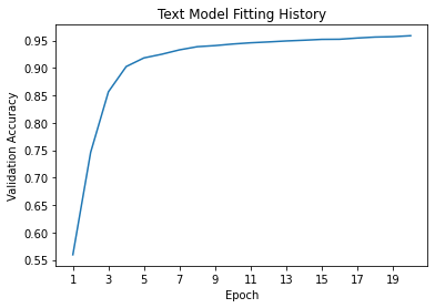
This is a bit better than before, but there’s still room for improvement. You’ll notice that despite the Functional API allowing for nonsequential models, we haven’t actually put this to use yet. So next, let’s try making a model that takes in both inputs. We’ll process them the same as before up until GlobalAveragePooling1D(), then concatenate them before applying a final Dense() layer. We can use utils.plot_model() again to visualize the model.
#create model that takes in both title and text as inputs

#two separate embedding layers for later plotting
title_embedding = layers.Embedding(size_vocabulary,output_dim=10,name="titleEmbedding")
text_embedding = layers.Embedding(size_vocabulary,output_dim=10,name="textEmbedding")

x = title_vectorize_layer(title_inputs)
x = title_embedding(x)
x = layers.Dropout(0.1)(x)
x = layers.GlobalAveragePooling1D()(x)

y = text_vectorize_layer(text_inputs)
y = text_embedding(y)
y = layers.Dropout(0.1)(y)
y = layers.GlobalAveragePooling1D()(y)

#combine branches of model into one output
main = layers.concatenate([x,y],axis=1)
outputs = layers.Dense(2,activation='softmax',name="fake")(main)

model = keras.Model(inputs=[title_inputs,text_inputs],outputs=outputs)

#visualize model
utils.plot_model(model)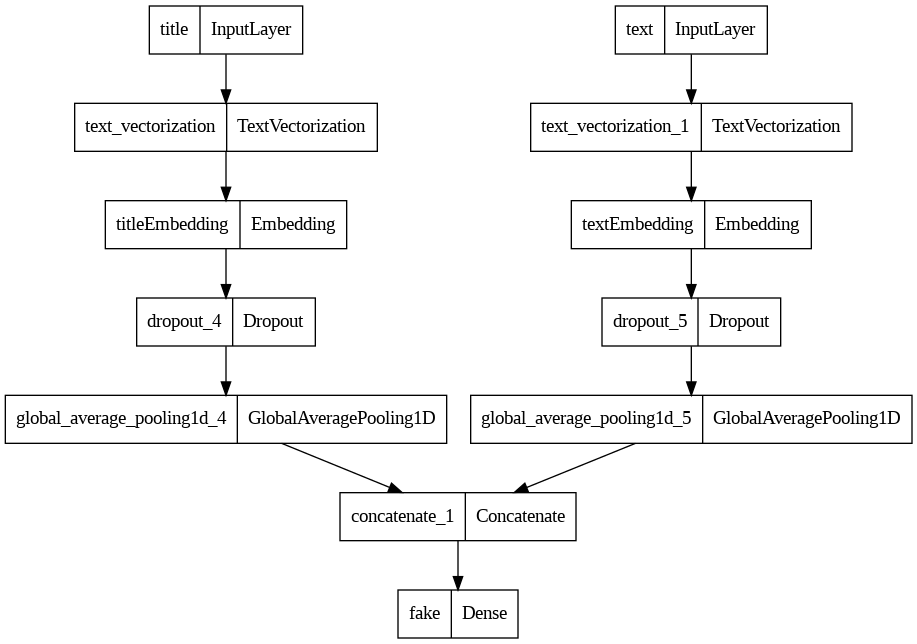
This model is more complicated than any of our earlier ones! Let’s see how it performs.
#compile model
sce = tf.keras.losses.SparseCategoricalCrossentropy(from_logits=False)

model.compile(optimizer='adam',
             loss = sce,
             metrics = ['accuracy'])

#train model
history = model.fit(train,epochs=20,validation_data=val)
Epoch 1/20
180/180 [==============================] - 12s 66ms/step - loss: 0.6716 - accuracy: 0.5938 - val_loss: 0.6392 - val_accuracy: 0.6516
Epoch 2/20
180/180 [==============================] - 13s 70ms/step - loss: 0.5838 - accuracy: 0.8621 - val_loss: 0.5260 - val_accuracy: 0.8856
Epoch 3/20
180/180 [==============================] - 12s 68ms/step - loss: 0.4676 - accuracy: 0.9316 - val_loss: 0.4177 - val_accuracy: 0.9336
Epoch 4/20
180/180 [==============================] - 12s 65ms/step - loss: 0.3736 - accuracy: 0.9445 - val_loss: 0.3401 - val_accuracy: 0.9460
Epoch 5/20
180/180 [==============================] - 12s 66ms/step - loss: 0.3074 - accuracy: 0.9520 - val_loss: 0.2864 - val_accuracy: 0.9507
Epoch 6/20
180/180 [==============================] - 12s 66ms/step - loss: 0.2604 - accuracy: 0.9579 - val_loss: 0.2476 - val_accuracy: 0.9551
Epoch 7/20
180/180 [==============================] - 12s 68ms/step - loss: 0.2255 - accuracy: 0.9620 - val_loss: 0.2182 - val_accuracy: 0.9602
Epoch 8/20
180/180 [==============================] - 12s 65ms/step - loss: 0.1983 - accuracy: 0.9658 - val_loss: 0.1950 - val_accuracy: 0.9636
Epoch 9/20
180/180 [==============================] - 12s 66ms/step - loss: 0.1764 - accuracy: 0.9690 - val_loss: 0.1761 - val_accuracy: 0.9669
Epoch 10/20
180/180 [==============================] - 12s 66ms/step - loss: 0.1583 - accuracy: 0.9723 - val_loss: 0.1604 - val_accuracy: 0.9702
Epoch 11/20
180/180 [==============================] - 12s 66ms/step - loss: 0.1431 - accuracy: 0.9750 - val_loss: 0.1470 - val_accuracy: 0.9716
Epoch 12/20
180/180 [==============================] - 12s 65ms/step - loss: 0.1303 - accuracy: 0.9767 - val_loss: 0.1356 - val_accuracy: 0.9729
Epoch 13/20
180/180 [==============================] - 12s 67ms/step - loss: 0.1189 - accuracy: 0.9789 - val_loss: 0.1256 - val_accuracy: 0.9751
Epoch 14/20
180/180 [==============================] - 12s 66ms/step - loss: 0.1091 - accuracy: 0.9807 - val_loss: 0.1169 - val_accuracy: 0.9769
Epoch 15/20
180/180 [==============================] - 12s 66ms/step - loss: 0.1003 - accuracy: 0.9824 - val_loss: 0.1092 - val_accuracy: 0.9780
Epoch 16/20
180/180 [==============================] - 12s 66ms/step - loss: 0.0923 - accuracy: 0.9836 - val_loss: 0.1024 - val_accuracy: 0.9798
Epoch 17/20
180/180 [==============================] - 12s 66ms/step - loss: 0.0855 - accuracy: 0.9852 - val_loss: 0.0962 - val_accuracy: 0.9809
Epoch 18/20
180/180 [==============================] - 12s 67ms/step - loss: 0.0794 - accuracy: 0.9860 - val_loss: 0.0907 - val_accuracy: 0.9818
Epoch 19/20
180/180 [==============================] - 13s 74ms/step - loss: 0.0737 - accuracy: 0.9870 - val_loss: 0.0857 - val_accuracy: 0.9822
Epoch 20/20
180/180 [==============================] - 12s 69ms/step - loss: 0.0687 - accuracy: 0.9879 - val_loss: 0.0812 - val_accuracy: 0.9833main_plot = plot_accuracies(history,"Combined Model")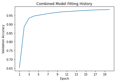
It looks like taking into account both the title and text of an article is best for determining whether or not it contains fake news. Just to be sure, let’s now test it on some testing data.
#import testing data
test_url = "https://github.com/PhilChodrow/PIC16b/blob/master/datasets/fake_news_test.csv?raw=true"
df = pd.read_csv(train_url)
test = make_dataset(df)
#evaluate main model on testing data
model.evaluate(test)225/225 [==============================] - 8s 35ms/step - loss: 0.0687 - accuracy: 0.9874[0.06867755204439163, 0.9873936772346497]So the model has 98.74% accuracy on the testing data.
Plotting Embeddings
When we put text through TextVectorization() and Embedding() layers, we end up with a weight for each word in the vocabulary in the form of a vector. In general an outlier means that the word has significant impact on the outcome. We can visualize these weights by graphing them. However, the output of the embedding layer in our model is 10 dimensions, which isn’t very convenient for plotting! We can use a PCA object imported from sklearn.decomposition to transform these weights into a two-dimensional vector, which we can then plot. Since we have two different vocabularies, we’ll make two plots.
pca = PCA(n_components=2)

def plot_weights(vocab,layer_name):
    #get weights from embedding layer and transform to visualizable data
    weights = model.get_layer(layer_name).get_weights()[0]
    weights = pca.fit_transform(weights)

    #plot data
    df = pd.DataFrame({"word":vocab,"x_0":weights[:,0],"x_1":weights[:,1]})
    return px.scatter(df,
                 x = "x_0",
                 y = "x_1",
                 #size = [2]*len(df),
                # size_max = 2,
                 hover_name = "word")

#get vocabulary lists from adapted TextVectorization layers
text_vocab = text_vectorize_layer.get_vocabulary()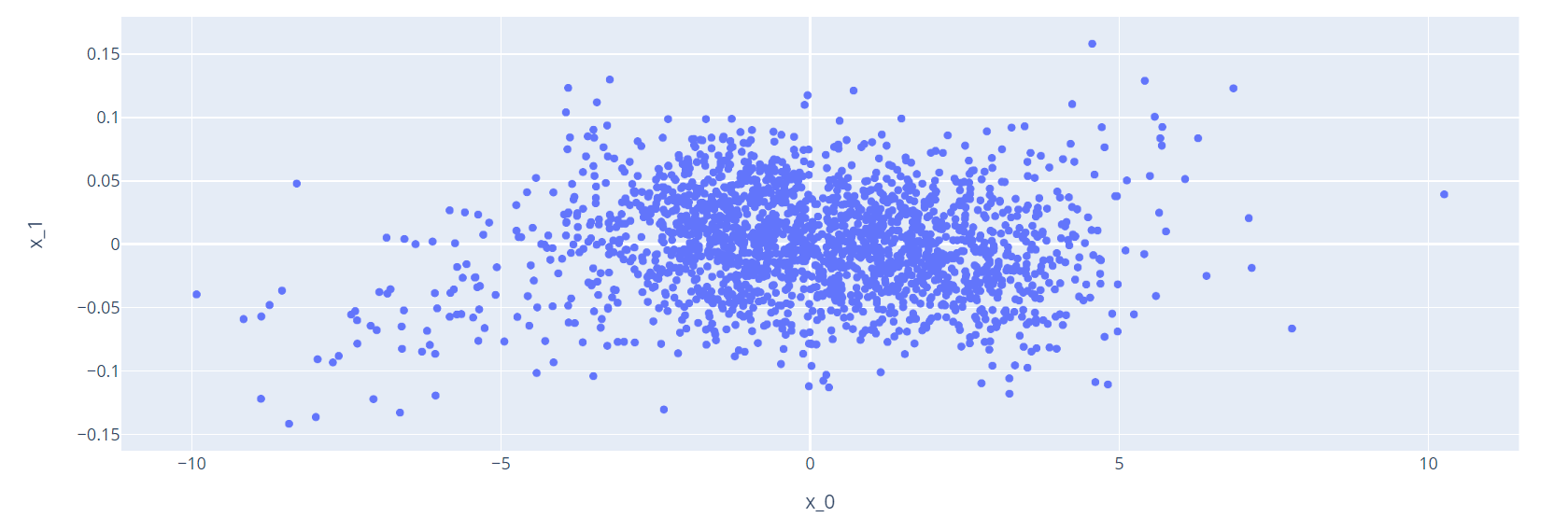
title_vocab = title_vectorize_layer.get_vocabulary()plot_weights(title_vocab,"titleEmbedding")The display is finicky when moving between Google Colab, Jupyter Notebook, and Quarto, so I’m inserting the graphs as figures. Unfortunately, they won’t be interactible, but we’ll do some analysis afterwards.
plot_weights(text_vocab,"textEmbedding")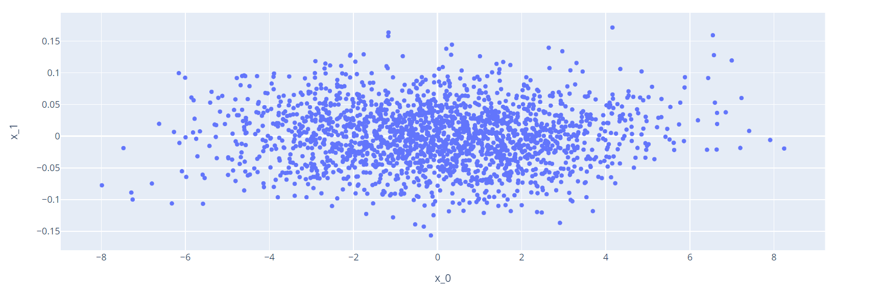
In the plot of title weights, the leftmost point is for “video,” and in the same region as an outlier is “breaking.” It’s possible that these correspond to news articles with less fake news, since breaking news articles are generally concerned with big undeniable events, and videos are often included in articles as evidence. In particular if “video” is mentioned in the title of an article, the contents are likely to be real footage.
Some outliers in the text weights plot include “trumps” and “obamas” on the rightmost side, whereas “obama” is on the leftmost side. Perhaps articles about politicians themselves tend to be more trustworthy, but news about their families (if we interpret “trumps” and “obamas” as such) can often contain speculation.